Working with samples

Samples in snompy are represented by instances of the Sample class. This page gives an overview of how samples are modelled in the finite dipole model (FDM) and point dipole model (PDM), with examples of how to create different types of Sample object in snompy.

Note

The way that different kinds of material interact with light can be described by their relative permittivity, \(\varepsilon\), which relates their absolute permittivity to the vacuum permittivity, \(\varepsilon_{0}\).

In the documentation for snompy, we will always use the term permittivity, to refer to the relative, not absolute, permitivitty.

Bulk samples

The simplest sort of sample to use for SNOM modelling is a bulk sample. These are infinite in the \(x\) and \(y\) directions, and are made of:

• a semi-infinite environment (sometimes called the superstrate), with permitivitty \(\varepsilon_{env}\) (which usually \(= 1\), for an air or vaccuum environment), stretching from \(z=0\) to \(+\infty\),

• a surface at \(z=0\), with a quasistatic reflection coefficient of

  \[\beta = \frac{\varepsilon_{sub} - \varepsilon_{env}}{\varepsilon_{sub} + \varepsilon_{env}},\]

• a semi-infinite substrate, with permitivitty \(\varepsilon_{sub}\), stretching from \(z=0\) to \(-\infty\).

The image below shows a cross-section of a simple bulk sample.

Creating bulk samples

In snompy, bulk samples can be created with the bulk_sample() function.

Let’s create a Si substrate as a first example. The permitivitty of Si in the mid-infrared (IR) is \(\varepsilon = 11.7\) [1], so we can create our sample as:

>>> import snompy
>>> eps_si = 11.7
>>> si = snompy.bulk_sample(eps_si)

Let’s take a look at some of the properties of the object we’ve just made:

>>> type(si)
<class 'snompy.sample.Sample'>
>>> si.eps_stack
array([ 1. +0.j, 11.7+0.j])

We can see that bulk_sample() creates an instance of the Sample class. The layers of the sample are represented by a complex array of \(\varepsilon\) values called eps_stack, which for our simple bulk sample has just two elements. The first of these corresponds to the environment, and the second to the substrate.

Hint

We didn’t have to specify the environment dielectric here, as we just used the default value of 1, but if needed bulk_sample() has an optional argument eps_env.

We can recover the quasistatic reflection coefficient of the sample using the function refl_coef_qs():

>>> beta_si = si.refl_coef_qs()
>>> beta_si
(0.84251968503937+0j)

Sometimes it’s more convenient to specify a sample using its quasistatic reflection coefficient, rather than its permitivitty. This can be done easily like:

>>> si_from_beta = snompy.bulk_sample(beta=beta_si)
>>> si_from_beta.eps_stack
array([ 1. +0.j, 11.7+0.j])

We can see that creating samples via eps_sub and beta lead to equivalent results.

Creating dispersive samples

Samples studied in SNOM experiments often have dispersive dielectric functions (which means their permitivitty changes depending on the frequency of the incident light). Let’s create a dispersive sample similar to poly(methyl methacrylate) (PMMA).

To begin with, we’ll define a dielectric function for our material (based loosely on reference [1]):

>>> import numpy as np
>>> wavenumber = np.linspace(1680, 1800, 128) * 1e2  # In units of m^-1
>>> eps_inf, centre_wavenumber, strength, width = 2, 1738e2, 4.2e8, 20e2
>>> eps_pmma = snompy.sample.lorentz_perm(
...     wavenumber,
...     nu_j=centre_wavenumber,
...     gamma_j=width,
...     A_j=strength,
...     eps_inf=eps_inf
... )

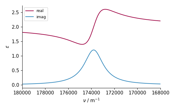
This is just a single Lorentzian oscillator. Let’s visualise it with a quick plot:

>>> import matplotlib.pyplot as plt
>>> fig, ax = plt.subplots()
>>> ax.plot(wavenumber, eps_pmma.real, label="real")
>>> ax.plot(wavenumber, eps_pmma.imag, label="imag")
>>> ax.set(
...     xlim=(wavenumber.max(), wavenumber.min()),
...     xlabel=r"$\nu$ / m$^{-1}$",
...     ylabel=r"$\varepsilon$",
... )
>>> ax.legend()
>>> fig.tight_layout()
>>> plt.show()

Now that we’ve created our dispersive dielectric function, we can pass it to our bulk_sample() function. We can also give it the wavenumber corresponding to each \(\varepsilon\) value as the optional argument nu_vac (which will be useful for some functions which depend on both parameters):

>>> pmma = snompy.bulk_sample(eps_pmma, nu_vac=wavenumber)

Let’s take a look at some of properties of this new sample:

>>> si.eps_stack.shape  # 2 layers with a single value for each
(2,)
>>> si.eps_stack
array([ 1. +0.j, 11.7+0.j])
>>> pmma.eps_stack.shape  # Each layer now has 128 elements
(2, 128)
>>> pmma.eps_stack[:, :4]  # First four values in each layer only
array([[1.        +0.j        , 1.        +0.j        ,
        1.        +0.j        , 1.        +0.j        ],
       [2.20736131+0.03514527j, 2.21053732+0.03628489j,
        2.21381045+0.03748023j, 2.21718504+0.03873494j]])

For our new sample, eps_stack still has 2 layers (corresponding to the environment and substrate), but it now also has 128 elements per layer. That’s one for each permitivitty value we used to generate it.

As before, we can use the function refl_coef_qs() to calculate the quasistatic reflection coefficient, which should have the same shape as eps_pmma and wavenumber:

>>> beta_pmma = pmma.refl_coef_qs()
>>> beta_pmma.shape
(128,)
>>> beta_pmma.shape == eps_pmma.shape == wavenumber.shape
True

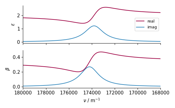
Let’s create another plot to visualise the dielectric function and quasistatic reflection coefficient together:

>>> fig, axes = plt.subplots(nrows=2, sharex=True)
>>> axes[0].plot(wavenumber, eps_pmma.real, label="real")
>>> axes[0].plot(wavenumber, eps_pmma.imag, label="imag")
>>> axes[0].set(ylabel=r"$\varepsilon$")
>>> axes[0].legend()
>>> axes[1].plot(wavenumber, beta_pmma.real)
>>> axes[1].plot(wavenumber, beta_pmma.imag)
>>> axes[1].set(
...     xlim=(wavenumber.max(), wavenumber.min()),
...     xlabel=r"$\nu$ / m$^{-1}$",
...     ylabel=r"$\beta$"
... )
>>> fig.tight_layout()
>>> plt.show()

Multilayer samples

Many samples can’t be modelled simply as an infinite substrate so snompy also supports multilayer samples, with more than two materials. Like bulk samples, these are infinite in the \(x\) and \(y\) directions. A multilayer sample with a number of layers, \(n_{\varepsilon}\), is made of:

• a semi-infinite environment, with permitivitty \(\varepsilon_{(0)}\), stretching from \(z=0\) to \(+\infty\),

  Note

  We use the symbol \(\varepsilon_{(0)}\) (with the subscript 0 in brackets) for the permitivitty of the top layer in a stack to distinguish it from \(\varepsilon_{0}\), the common symbol for vacuum permittivity.

• one or more sandwiched layers, with permitivitties \(\varepsilon_{i}\) and finite thicknesses \(t_{i-1}\) (for \(i=1, ..., n_{\varepsilon} - 2\)),

  Note

  The indices for the corresponding \(\varepsilon\) and \(t\) values are offset by 1, because the first \(\varepsilon\) layer (\(\varepsilon_{(0)}\)) is semi-infinite and has no thickness. This could be accounted for by starting the \(t\) indexing at 1, but we prefer to start at 0 to match the indexing of Python arrays.

• two or more interfaces at the boundaries between layers, with quasistatic reflection coefficients of

  \[\beta_i = \frac{\varepsilon_{i+1} - \varepsilon_{i}}{\varepsilon_{i+1} + \varepsilon_{i}},\]

• a semi-infinite substrate, with permitivitty \(\varepsilon_{n_{\varepsilon} - 1}\), stretching from the depth of the lowest interface to \(-\infty\).

The image below shows a cross-section of a multilayer sample with \(n_{\varepsilon} = 4\).

Creating multilayer samples

In snompy, multilayer samples can be created by directly initializing an instance of the Sample class.

Let’s create sample of 100 nm of Si, suspended over air as a first example.

>>> t_si = 100e-9
>>> eps_air = 1.0
>>> suspended_si = snompy.Sample(
...     eps_stack=(eps_air, eps_si, eps_air),
...     t_stack=(t_si,)
... )

Note

Even though t_stack has only one value here, we still must pass a list rather than a single value to the Sample object. That’s because snompy always uses the first axis of t_stack (and eps_stack and beta_stack) to store the different layers of the stack.

The top and bottom dielectric layers in eps_stack have no finite thickness, so eps_stack must always be 2 longer than t_stack along the first axis.

Now let’s compare our new sample with the bulk Si sample we created earlier:

>>> si.multilayer  # Bulk Si
False
>>> si.eps_stack
array([ 1. +0.j, 11.7+0.j])
>>> si.beta_stack
array([0.84251969+0.j])
>>> si.t_stack
array([], dtype=float64)
>>> suspended_si.multilayer  # Suspended Si
True
>>> suspended_si.eps_stack
array([ 1. +0.j, 11.7+0.j,  1. +0.j])
>>> suspended_si.beta_stack
array([ 0.84251969+0.j, -0.84251969+0.j])
>>> suspended_si.t_stack
array([1.e-07])

As well as the eps_stack we looked at before, we now also look at beta_stack, which shows the quasistatic reflection coefficients between each interface, and t_stack, which shows the thickness of each sandwiched dielectric layer. This makes it clear that bulk samples are actually just a special case of multilayer samples, with only two dielectric layers and an empty array for t_stack.

Creating dispersive samples with varying thickness

In the section on bulk samples above, we showed how you can create a single Sample object with an array of permitivitties to represent a dispersive sample.

Let’s show the same process for multilayer samples, by creating a thin layer of 50 nm of PMMA on Si. We already defined permitivitties for Si and PMMA above, so we can reuse the same values here:

>>> t_pmma = 50e-9
>>> pmma_si = snompy.Sample(
...     eps_stack=(eps_air, eps_pmma, eps_si),
...     t_stack=(t_pmma,),
...     nu_vac=wavenumber,
... )

Remember that eps_pmma is a 128-value numpy array, but eps_air and eps_si are scalar values. Let’s compare the shape of the resulting eps_stack with the shapes of the inputs:

>>> [np.shape(eps) for eps in (eps_air, eps_pmma, eps_si)]
[(), (128,), ()]
>>> pmma_si.eps_stack.shape
(3, 128)
>>> pmma_si.eps_stack[:, :4]
array([[ 1.        +0.j        ,  1.        +0.j        ,
         1.        +0.j        ,  1.        +0.j        ],
       [ 2.20736131+0.03514527j,  2.21053732+0.03628489j,
         2.21381045+0.03748023j,  2.21718504+0.03873494j],
        [11.7       +0.j        , 11.7       +0.j        ,
         11.7       +0.j        , 11.7       +0.j        ]])

We can see that snompy automatically pads the input permitivitties so that each layer of the stack has the same shape. This same process also works for beta_stack and t_stack.

What if we want to also vary the thickness of the PMMA? As we did for the permitivitty, we can create a single snompy.sample.Sample object with a range of thickness values. In fact, snompy takes advantage of numpy broadcasting, meaning that one sample can have both a range of thickness values and a range of permitivitties, as long as all the input arrays broadcast nicely with each other.

We can check whether two arrays broadcast nicely by adding them together. If we don’t get an error, the shape of the resulting array should tell us our broadcast shape:

>>> t_pmma_varied = np.linspace(1, 400, 32) * 1e-9
>>> t_pmma_varied = t_pmma_varied[:, np.newaxis]  # Add new axis for broadcasting
>>> (eps_pmma + t_pmma_varied).shape  # Error if arrays don't broadcast
(32, 128)

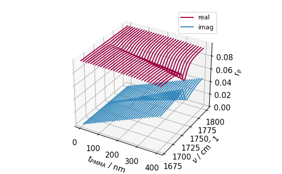
Now we know our arrays broadcast nicely, let’s show the advantage of broadcasting, by calculating the far-field reflection spectrum for all 32 thicknesses of PMMA in one vectorized calculation (see Far-field reflections for more detail):

>>> pmma_si_varied = snompy.Sample(
...     eps_stack=(eps_air, eps_pmma, eps_si),
...     t_stack=(t_pmma_varied,),
...     nu_vac=wavenumber,
... )
>>> theta_in = np.deg2rad(70)  # Incident angle of light
>>> r_p = pmma_si_varied.refl_coef(theta_in=theta_in)
>>> r_p.shape
(32, 128)

We can see that our far-field reflection coefficient r_p has the same shape as the broadcast array from our inputs. Let’s plot this in 3D to see what this looks like:

>>> fig, ax = plt.subplots(subplot_kw={"projection":"3d"})
>>> for i, t in enumerate(t_pmma_varied * 1e9):
...     l_real, = ax.plot(
...         wavenumber * 1e-2,
...         r_p[i].real,
...         t,
...         zdir="x",
...         c='C0'
...     )
...     l_imag, = ax.plot(
...         wavenumber * 1e-2,
...         r_p[i].imag,
...         t,
...         zdir="x",
...         c='C1'
...     )
>>> ax.set(
...    xlabel=r"$t_{PMMA}$ / nm",
...    ylabel=r"$\nu$ / cm$^-1$",
...    zlabel=r"$r_p$",
... )
>>> ax.legend((l_real, l_imag), ("real", "imag"))
>>> fig.tight_layout()
>>> plt.show()

Momentum-dependence

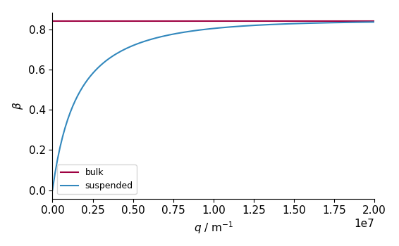
For multilayer samples, calculating the effective quasistatic reflection coefficient from the whole stack becomes more complicated, as it depends on the in-plane momentum, \(q\), of the incident light. This can be accounted for with the optional argument q to refl_coef_qs().

To show this, let’s plot \(\beta\) as a function of \(q\) for both our bulk and suspended Si samples:

>>> q = np.linspace(0, 2 / t_si, 128)
>>> beta_si_q = si.refl_coef_qs(q)
>>> beta_suspended_si_q = suspended_si.refl_coef_qs(q)
>>> fig, ax = plt.subplots()
>>> ax.plot(q, beta_si_q.real, label="bulk")
>>> ax.plot(q, beta_suspended_si_q.real, label="suspended")
>>> ax.set(
...    xlim=(q.min(), q.max()),
...    xlabel=r"$q$ / m$^{-1}$",
...    ylabel=r"$\beta$"
... )
>>> ax.legend()
>>> fig.tight_layout()
>>> plt.show()

For this reason, the models of effective polarizability in snompy (the FDM and PDM) have different methods for bulk and multilayer samples.

References

[1] (1,2)

L. Mester, A. A. Govyadinov, S. Chen, M. Goikoetxea, and R. Hillenbrand, “Subsurface chemical nanoidentification by nano-FTIR spectroscopy,” Nat. Commun., vol. 11, no. 1, p. 3359, Dec. 2020, doi: 10.1038/s41467-020-17034-6.