Far-field reflections

In Basics of SNOM modelling, we showed the image below to explain why far-field reflections are important for modelling SNOM measurements.

We showed that the detected SNOM signal, \(\sigma_n\), depends on the effective polarizability, \(\alpha_{eff, n}\), and a far-field reflection term, \((1 + c_r r)^2\), as

(1)\[\sigma_n = (1 + c_r r)^2 \alpha_{eff, n},\]

where \(r\) is the the far-field, Fresnel reflection coefficient and \(c_r\) is an empirical factor that describes the detected strength of the reflected light compared to the incident light.

On this page, we’ll provide some background on what the far-field, Fresnel reflection coefficient is, and give an example of how it can be calculated using snompy.

Fresnel reflection coefficient

Bulk samples

The Fresnel reflection coefficient relates the strength of a reflected light beam to the strength of the incident beam. For a bulk sample it can be calculated simply.

The image below shows a diagram of a simple reflection from a bulk sample. An incident light beam with electric field \(E_{in}\) hits the sample surface. Then, part of the beam is reflected with field \(E_{r}\), and part is transmitted with field \(E_{t}\).

The angle of the reflected beam to the surface normal, \(\theta_r\), is the same as the angle of incidence, \(\theta_{in}\), and the angle of the transmitted beam can be found from Snell’s law as

\[n_0 \sin(\theta_{in}) = n_1 \sin(\theta_t),\]

where \(n_0\) and \(n_1\) are the refractive indices of the environment and the sample.

Hint

In general, the refractive index, \(n\), can be found from the permittivity as \(n = \sqrt{\varepsilon}\) for non-magnetic materials.

The value of the reflection coefficient depends on the angle and polarization, \(P\), of the incident light as

\[\begin{split}r = \begin{cases} r_p = \frac{n_0 \cos(\theta_{in} - n_1 \cos(\theta_{r})}{n_0 \cos(\theta_{in} + n_1 \cos(\theta_{r})}, & \text{for} \ P = p\\ r_s = \frac{n_1 \cos(\theta_{in} - n_0 \cos(\theta_{r})}{n_1 \cos(\theta_{in} + n_0 \cos(\theta_{r})}, & \text{for} \ P = s\\ \end{cases}\end{split}\]

Hint

The term p polarization refers to electric fields that are parallel to the plane of incidence (as shown in the drawing above). The term s polarisation comes from the German word senkrecht, and refers to electric fields that are perpendicular to the plane of incidence. In SNOM measurements we almost always use p polarisation.

Multilayer samples

For multilayer samples, calculating the reflection coefficient becomes more complicated, as we must account for reflections from multiple surfaces. In snompy we use the transfer matrix method to calculate reflection and transmission coefficients from multilayer samples [1].

Accounting for far-field in SNOM simulations

The most common use for the far-field reflection coefficient in snompy is to calculate the far-field factor \((1 + c_r r)^2\) (as in equation (1)). In this section we’ll show a worked example, by simulating a SNOM spectrum from a layer of poly(methyl methacrylate) (PMMA) on Si.

Far-field factor from a bulk reference

We’ll normalize our spectrum to bulk Si. Let’s start by creating a Sample object for our reference (see Working with samples for a guide to sample creation):

>>> import snompy
>>> eps_si = 11.7
>>> si = snompy.bulk_sample(eps_si)

The single permitivitty value \(\varepsilon = 11.7\) for Si, is relatively constant across most of the mid-infrared [2].

Now let’s calculate our far-field factor. We’ll need to define some experimental constants here:

• The fresnel reflection coefficient depends on the angle of incidence of the far-field beam, \(\theta_{in}\): For most SNOM experiments this is around 60°.

• The empirical factor, \(c_r\), will vary from microscope to microscope and the value should be chosen to best fit the data. We’ll use a value of \(c_r = 0.9\).

>>> import numpy as np
>>> theta_in = np.deg2rad(60)  # Angle must be in radians
>>> c_r = 0.9
>>> r_si = si.refl_coef(theta_in=theta_in)
>>> fff_si = (1 + c_r * r_si)**2  # Far-field factor
>>> fff_si
(1.173379279716862+0j)

Note

The method refl_coef() has an optional argument polarization which can be either “s” or “p”. Here we use the default p polarization which is most common for SNOM experiments.

Far-field factor from a dispersive sample

Now let’s do the same for our PMMA. First let’s create a model for the permitivitty (based loosely on [2]):

>>> wavenumber = np.linspace(1680, 1800, 128) * 1e2  # In units of m^-1
>>> eps_inf, centre_wavenumber, strength, width = 2, 1738e2, 4.2e8, 20e2
>>> eps_pmma = snompy.sample.lorentz_perm(
...     wavenumber,
...     nu_j=centre_wavenumber,
...     gamma_j=width,
...     A_j=strength,
...     eps_inf=eps_inf
... )

Now we can create our sample. Let’s make it 500 nm thick, and we’ll define the environment to be air with \(\varepsilon_{env} = 1\) (this was done automatically for Si by bulk_sample() above).

>>> eps_air = 1.0
>>> t_pmma = 500e-9
>>> pmma_si = snompy.Sample(
...     eps_stack=(eps_air, eps_pmma, eps_si),
...     t_stack=(t_pmma,),
...     nu_vac=wavenumber,
... )

We’ll use the same values for \(c_r\) and \(\theta_{in}\) that we used for our reference (this is important so it’s a fair comparison). Let’s calculate our far-field factor:

>>> r_pmma_si = pmma_si.refl_coef(theta_in=theta_in)
>>> fff_pmma_si = (1 + c_r * r_pmma_si)**2
>>> wavenumber.shape == r_pmma_si.shape == fff_pmma_si.shape
True

We can see that our reflection coefficient and far-field factor have the same shape as our wavenumber array (i.e. one value per wavenumber).

Normalized SNOM spectra with far-field factor

Now we’ve found our far-field factors, we can calculate the effective polarizability from our sample and reference and combine them together using:

(2)\[\eta_n = \frac{\sigma_n}{\sigma_n^{\text{(ref)}}} = \frac{(1 + c_r r)^2 \alpha_{eff, n}} {(1 + c_r r^{\text{(ref)}})^2 \alpha_{eff, n}^{\text{(ref)}}}\]

(see Normalization for why we use \(\eta_n\) rather than \(\sigma_n\)).

Let’s use the finite dipole method to calculate our effective polarizabilities and SNOM contrast. We’ll also create an array eta_uncorr, which will show the results if we didn’t account for the far-field factors:

>>> fdm_params = dict(A_tip=20e-9, n=3)
>>> alpha_eff_si = snompy.fdm.eff_pol_n(sample=si, **fdm_params)
>>> alpha_eff_pmma_si = snompy.fdm.eff_pol_n(
...     sample=pmma_si,
...     **fdm_params,
... )
>>> eta_uncorr = alpha_eff_pmma_si / alpha_eff_si
>>> eta = (
...     (fff_pmma_si * alpha_eff_pmma_si)
...     / (fff_si * alpha_eff_si)
... )

Finally, let’s make a plot to show our results. This is quite a busy plot, so let’s break it up into steps. First we’ll set up our axes and define some colours:

>>> import matplotlib.pyplot as plt
>>> wavenumber_per_cm = wavenumber * 1e-2
>>> c_re, c_im = "C0", "C1"
>>> c_s, c_phi = "C2", "C3"
>>> ls_sample, ls_ref = "-", "--"
>>> ls_corr, ls_uncorr = "-.", ":"
>>> fig, axes = plt.subplots(nrows=3, sharex=True)
>>> axes[-1].set(
...    xlabel=r"$\nu$ / cm$^{-1}$",
...    xlim=(wavenumber_per_cm.max(), wavenumber_per_cm.min()),
... )

Now we’ll plot our parameters one by one:

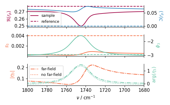
• The real part of our reflection coefficients:

  >>> # Plot real part
  >>> ax_r_re = axes[0]
  >>> ax_r_re.plot(
  ...     wavenumber_per_cm,
  ...     r_pmma_si.real,
  ...     c=c_re,
  ...     ls=ls_sample,
  ...     label="sample",
  ... )
  >>> ax_r_re.axhline(
  ...     r_si.real,
  ...     c=c_re,
  ...     ls=ls_ref,
  ...     label="reference"
  ... )
  >>> ax_r_re.set_ylabel(r"$\Re(r_p)$", c=c_re)
  >>> ax_r_re.legend(loc="lower left")
  

• The imaginary part of our reflection coefficients:

  >>> ax_r_im = ax_r_re.twinx()
  >>> ax_r_im.spines["right"].set_visible(True)
  >>> ax_r_im.plot(
  ...     wavenumber_per_cm,
  ...     r_pmma_si.imag,
  ...     c=c_im,
  ...     ls=ls_sample,
  ... )
  >>> ax_r_im.axhline(r_si.imag, c=c_im, ls=ls_ref)
  >>> ax_r_im.set_ylabel(r"$\Im(r_p)$", c=c_im)
  

• The magnitude of our effective polarizabilities:

  >>> ax_alpha_s = axes[1]
  >>> ax_alpha_s.plot(
  ...     wavenumber_per_cm,
  ...     np.abs(alpha_eff_pmma_si),
  ...     c=c_s,
  ...     ls=ls_sample,
  ... )
  >>> ax_alpha_s.axhline(
  ...     np.abs(alpha_eff_si),
  ...     c=c_s,
  ...     ls=ls_ref,
  ... )
  >>> ax_alpha_s.set_ylabel(r"$s_3$", c=c_s)
  

• The phase of our effective polarizabilities:

  >>> ax_alpha_phi = ax_alpha_s.twinx()
  >>> ax_alpha_phi.spines["right"].set_visible(True)
  >>> ax_alpha_phi.plot(
  ...     wavenumber_per_cm,
  ...     np.angle(alpha_eff_pmma_si),
  ...     c=c_phi,
  ...     ls=ls_sample,
  ... )
  >>> ax_alpha_phi.axhline(
  ...     np.angle(alpha_eff_si),
  ...     c=c_phi,
  ...     ls=ls_ref,
  ... )
  >>> ax_alpha_phi.set_ylabel(r"$\phi_3$", c=c_phi)
  

• The magnitude of our near field contrast:

  >>> ax_eta_s = axes[2]
  >>> ax_eta_s.plot(
  ...     wavenumber_per_cm,
  ...     np.abs(eta),
  ...     c=c_s,
  ...     ls=ls_corr,
  ...     label="far-field",
  ... )
  >>> ax_eta_s.plot(
  ...     wavenumber_per_cm,
  ...     np.abs(eta_uncorr),
  ...     c=c_s,
  ...     ls=ls_uncorr,
  ...     label="no far-field",
  ... )
  >>> ax_eta_s.set_ylabel(r"$|\eta_3|$", c=c_s)
  >>> ax_eta_s.legend(loc="upper left")
  

• The phase of our near field contrast:

  >>> ax_eta_phi = ax_eta_s.twinx()
  >>> ax_eta_phi.spines["right"].set_visible(True)
  >>> ax_eta_phi.plot(
  ...     wavenumber_per_cm,
  ...     np.angle(eta),
  ...     c=c_phi,
  ...     ls=ls_corr,
  ... )
  >>> ax_eta_phi.plot(
  ...     wavenumber_per_cm,
  ...     np.angle(eta_uncorr),
  ...     c=c_phi,
  ...     ls=ls_uncorr,
  ... )
  >>> ax_eta_phi.set_ylabel(r"$\arg(\eta_3)$", c=c_phi)
  

Finally, let’s show our finished figure:

>>> fig.tight_layout()
>>> plt.show()

References

[1]

20. Zhan, X. Shi, Y. Dai, X. Liu, and J. Zi, “Transfer matrix method for optics in graphene layers,” J Phys. Condens. Matter, vol. 25, no. 21, p. 215301, May 2013, doi: 10.1088/0953-8984/25/21/215301.

[2] (1,2)

12. Mester, A. A. Govyadinov, S. Chen, M. Goikoetxea, and R. Hillenbrand, “Subsurface chemical nanoidentification by nano-FTIR spectroscopy,” Nat. Commun., vol. 11, no. 1, p. 3359, Dec. 2020, doi: 10.1038/s41467-020-17034-6.