Introduction

The main purpose of snompy is to provide functions to calculate the effective polarizability, \(\alpha_{eff}\), of a SNOM tip and a sample, which can be used to predict contrast in SNOM measurements. It also contains other useful features for SNOM modelling, such as an implementation of the transfer matrix method for calculating far-field reflection coefficients of multilayer samples, and code for simulating lock-in amplifier demodulation of arbitrary functions.

Below on this page are some example scripts, showing idiomatic usage of snompy. If you already know how the finite dipole model (FDM) or point dipole model (PDM) works, these might be enough to get started with this package. You can also refer to the detailed explanations of the functions used in the API reference. The rest of this guide will take you through the workings of the two models, and also give tips on how the models can be used to help analyse SNOM data.

Installation

Using pip:

pip install snompy

Using conda:

conda install -c conda-forge snompy

Useful third-party packages

The examples in this guide rely heavily on numpy, a Python package for eficient numerical computation, which should be installed automatically when you install snompy. To follow along, it might also be helpful to install matplotlib, a Python package for data visualisation, and scipy, a Python package for scientific computation. These can be installed like:

pip install matplotlib scipy

or for conda users:

conda install -c conda-forge matplotlib scipy

Usage examples

The examples on this page are intended to give a taste of what snompy can do, as well as to model idiomatic use of the package. We’ve deliberately left out detailed explanations from this section, so don’t worry if you don’t understand what’s going on here yet! The following pages of this guide should take you through the concepts needed to understand these scripts.

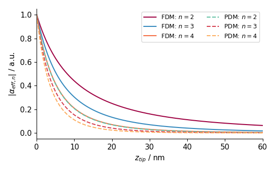
Approach curve on silicon

This example uses both the FDM and PDM to calculate the decay of the SNOM amplitude, \(s_n \propto \alpha_{eff, n}\), for different demodulation harmonics, \(n\) as the SNOM tip is moved in the \(z\) direction, away from a sample of bulk silicon.

import matplotlib.pyplot as plt
import numpy as np

import snompy

# Set some experimental parameters for an AFM approach curve
z_tip = np.linspace(0, 60e-9, 512)  # Define an approach curve
A_tip = 20e-9  # AFM tip tapping amplitude
harmonics = np.array([2, 3, 4])  # Harmonics for demodulation
eps_Si = 11.7  # Si permitivitty in the mid-infrared
sample = snompy.bulk_sample(eps_sub=eps_Si)  # Sample object

# Calculate the effective polarizability using FDM and PDM
alpha_eff_fdm = snompy.fdm.eff_pol_n(
    sample=sample,
    A_tip=A_tip,
    n=harmonics,
    z_tip=z_tip[:, np.newaxis],  # newaxis added for array broadcasting
)
alpha_eff_pdm = snompy.pdm.eff_pol_n(
    sample=sample,
    A_tip=A_tip,
    n=harmonics,
    z_tip=z_tip[:, np.newaxis],  # newaxis added for array broadcasting
)

# Normalize to value at z_tip = 0
alpha_eff_fdm /= alpha_eff_fdm[0]
alpha_eff_pdm /= alpha_eff_pdm[0]

# Plot output
fig, ax = plt.subplots()
z_nm = z_tip * 1e9  # For neater plotting
ax.plot(z_nm, np.abs(alpha_eff_fdm), label=[f"FDM: $n = ${n}" for n in harmonics])
ax.plot(
    z_nm, np.abs(alpha_eff_pdm), label=[f"PDM: $n = ${n}" for n in harmonics], ls="--"
)
ax.set(
    xlabel=r"$z_{tip}$ / nm",
    ylabel=r"$|\alpha_{eff, n}|$ / a.u.",
    xlim=(z_nm.min(), z_nm.max()),
)
ax.legend(ncol=2)
fig.tight_layout()
plt.show()

Thickness-dependent PMMA spectra

This more involved example uses the a multilayer FDM to simulate a SNOM spectrum from a thin layer of poly(methyl methacrylate) (PMMA) on silicon, for different thicknesses of PMMA, and normalises the signal to a reference spectrum taken from bulk gold. It also includes the effects of the far-field reflection coefficient of the sample on the observed SNOM spectra.

import matplotlib.pyplot as plt
import numpy as np
from matplotlib.colors import Normalize

import snompy

# Set some experimental parameters
A_tip = 20e-9  # AFM tip tapping amplitude
r_tip = 30e-9  # AFM tip radius of curvature
L_tip = 350e-9  # Semi-major axis length of ellipsoid tip model
n = 3  # Harmonic for demodulation
theta_in = np.deg2rad(60)  # Light angle of incidence
c_r = 0.3  # Experimental weighting factor
nu_vac = np.linspace(1680, 1800, 128) * 1e2  # Vacuum wavenumber
method = "Q_ave"  # The FDM method to use

# Semi-infinite superstrate and substrate
eps_air = 1.0
eps_Si = 11.7  # Si permitivitty in the mid-infrared

# Very simplified model of PMMA dielectric function based on ref [1] below
eps_pmma = snompy.sample.lorentz_perm(
    nu_vac, nu_j=1738e2, gamma_j=20e2, A_j=4.2e8, eps_inf=2
)
t_pmma = np.geomspace(1, 35, 32) * 1e-9  # A range of thicknesses
sample_pmma = snompy.Sample(
    eps_stack=(eps_air, eps_pmma, eps_Si),
    t_stack=(t_pmma[:, np.newaxis],),
    nu_vac=nu_vac,
)

# Model of Au dielectric function from ref [2] below
eps_Au = snompy.sample.drude_perm(nu_vac, nu_plasma=7.25e6, gamma=2.16e4)
sample_Au = snompy.bulk_sample(eps_sub=eps_Au, eps_env=eps_air, nu_vac=nu_vac)

# Measurement
alpha_eff_pmma = snompy.fdm.eff_pol_n(
    sample=sample_pmma, A_tip=A_tip, n=n, r_tip=r_tip, L_tip=L_tip, method=method
)
r_coef_pmma = sample_pmma.refl_coef(theta_in=theta_in)
sigma_pmma = (1 + c_r * r_coef_pmma) ** 2 * alpha_eff_pmma

# Gold reference
alpha_eff_Au = snompy.fdm.eff_pol_n(
    sample=sample_Au, A_tip=A_tip, n=n, r_tip=r_tip, L_tip=L_tip, method=method
)
r_coef_Au = sample_Au.refl_coef(theta_in=theta_in)
sigma_Au = (1 + c_r * r_coef_Au) ** 2 * alpha_eff_Au

# Normalised complex scattering
eta_n = sigma_pmma / sigma_Au

# Plot output
fig, axes = plt.subplots(nrows=2, sharex=True)

# For neater plotting
nu_per_cm = nu_vac * 1e-2
t_nm = t_pmma * 1e9

SM = plt.cm.ScalarMappable(
    cmap=plt.cm.Spectral_r, norm=Normalize(vmin=t_nm.min(), vmax=t_nm.max())
)  # This maps thickness to colour

for t, sigma in zip(t_nm, eta_n):
    c = SM.to_rgba(t)
    axes[0].plot(nu_per_cm, np.abs(sigma), c=c)
    axes[1].plot(nu_per_cm, np.angle(sigma), c=c)

axes[0].set_ylabel(r"$s_{" f"{n}" r"}$ / a.u.")
axes[1].set(
    xlabel=r"$\nu$ / cm$^{-1}$",
    ylabel=r"$\phi_{" f"{n}" r"}$ / radians",
    xlim=(nu_per_cm.max(), nu_per_cm.min()),
)
fig.tight_layout()
cbar = fig.colorbar(SM, ax=axes, label="PMMA thickness / nm")
plt.show(block=False)

(The dielectric function of PMMA in the above example was based roughly on reference [1], and the dielectric function of gold was taken from reference [2]).

References

[1]

L. Mester, A. A. Govyadinov, S. Chen, M. Goikoetxea, and R. Hillenbrand, “Subsurface chemical nanoidentification by nano-FTIR spectroscopy,” Nat. Commun., vol. 11, no. 1, p. 3359, Dec. 2020, doi: 10.1038/s41467-020-17034-6.

[2]

M. A. Ordal et al., “Optical properties of the metals Al, Co, Cu, Au, Fe, Pb, Ni, Pd, Pt, Ag, Ti, and W in the infrared and far infrared,” Appl. Opt., vol. 22, no. 7, p. 1099, Apr. 1983, doi: 10.1364/AO.22.001099.