Approach curve on silicon

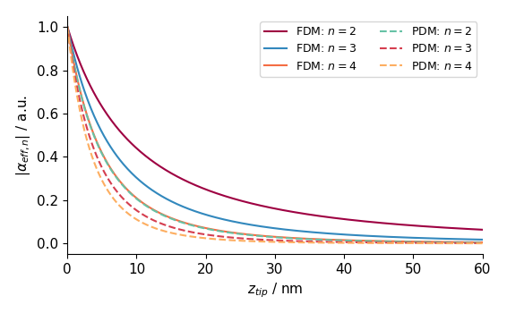
This example uses both the FDM and PDM to calculate the decay of the SNOM amplitude, \(s_n \propto \alpha_{eff, n}\), for different demodulation harmonics, \(n\) as the SNOM tip is moved in the \(z\) direction, away from a sample of bulk silicon.

import matplotlib.pyplot as plt
import numpy as np

import snompy

# Set some experimental parameters for an AFM approach curve
z_tip = np.linspace(0, 60e-9, 512)  # Define an approach curve
A_tip = 20e-9  # AFM tip tapping amplitude
harmonics = np.array([2, 3, 4])  # Harmonics for demodulation
eps_Si = 11.7  # Si permitivitty in the mid-infrared
sample = snompy.bulk_sample(eps_sub=eps_Si)  # Sample object

# Calculate the effective polarizability using FDM and PDM
alpha_eff_fdm = snompy.fdm.eff_pol_n(
    sample=sample,
    A_tip=A_tip,
    n=harmonics,
    z_tip=z_tip[:, np.newaxis],  # newaxis added for array broadcasting
)
alpha_eff_pdm = snompy.pdm.eff_pol_n(
    sample=sample,
    A_tip=A_tip,
    n=harmonics,
    z_tip=z_tip[:, np.newaxis],  # newaxis added for array broadcasting
)

# Normalize to value at z_tip = 0
alpha_eff_fdm /= alpha_eff_fdm[0]
alpha_eff_pdm /= alpha_eff_pdm[0]

# Plot output
fig, ax = plt.subplots()
z_nm = z_tip * 1e9  # For neater plotting
ax.plot(z_nm, np.abs(alpha_eff_fdm), label=[f"FDM: $n = ${n}" for n in harmonics])
ax.plot(
    z_nm, np.abs(alpha_eff_pdm), label=[f"PDM: $n = ${n}" for n in harmonics], ls="--"
)
ax.set(
    xlabel=r"$z_{tip}$ / nm",
    ylabel=r"$|\alpha_{eff, n}|$ / a.u.",
    xlim=(z_nm.min(), z_nm.max()),
)
ax.legend(ncol=2)
fig.tight_layout()
plt.show()