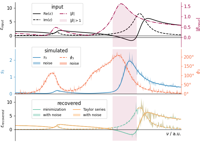
Inverting the FDM

This example inverts the finite dipole model (FDM) using scipy’s optimize.minimize and by using a built-in method provided by snompy that uses a Taylor series representation of the effective polarizability. The taylor series representation only works for samples with weak light matter interaction.

import matplotlib.pyplot as plt
import numpy as np
from matplotlib.ticker import StrMethodFormatter
from scipy.optimize import minimize

import snompy


def minimization_function(eps_re_im, alpha_eff_n, fdm_params):
    """
    Returns the absolute difference between `alpha_eff_n` and the effective
    polarizability generated from permitivitty `eps_re_im` with `fdm_params`.

    Parameters
    ----------
    eps_re_im : array_like
        Length 2 array with the real part in the first index and the imaginary
        part in the second. The imaginary part is constrained to be positive.
    alpha_eff_n : float
        The target effective polarizability.
    fdm_params : dict
        Parameters for the finite difference method (FDM).

    Returns
    -------
    float
        Absolute difference between `alpha_eff_n` and calculated effective
        polarizability.

    Notes
    -----
    `eps_re_im` is not a complex number, but a length 2 array with the real
    part in the first index and the imaginary part in the second (because
    `scipy.optimize.minimize` only works on real arrays).
    """
    eps = eps_re_im[0] + 1j * np.abs(eps_re_im[1])
    alpha_eff_n_test = snompy.fdm.eff_pol_n(snompy.bulk_sample(eps), **fdm_params)
    return np.abs(alpha_eff_n - alpha_eff_n_test)


def invert_by_minimization(alpha_eff_n, initial_guess, fdm_params):
    """
    Uses `scipy.optimize.minimize` and `minimization_function` to find the
    permitivitty values that lead to `alpha_eff_n`, using the finite
    difference method (FDM) with `fdm_params`.

    Parameters
    ----------
    alpha_eff_n : array_like
        The target effective polarizabilities.
    initial_guess : array_like
        Initial guess for the permitivitty values. Should be the same shape
        as `alpha_eff_n`.
    fdm_params : dict
        Parameters for the finite difference method (FDM).

    Returns
    -------
    array_like
        Permitivitty values that lead to `alpha_eff_n`.

    Notes
    -----
    Internally this function loops through the individual values of
    `alpha_eff_n` as `scipy.optimize.minimize` is not natively vectorized.
    The returned values of permitivitty are constrained to have positive
    imaginary parts.
    """
    eps = np.zeros_like(alpha_eff_n)
    for inds in np.ndindex(eps.shape):
        res = minimize(
            minimization_function,
            (initial_guess[inds].real, initial_guess[inds].imag),
            args=(alpha_eff_n[inds], fdm_params),
        )
        eps[inds] = res.x[0] + 1j * np.abs(res.x[1])
    return eps


# Choose some parameters for the FDM
fdm_params = dict(A_tip=30e-9, n=3)

# Simulate a dielectric function with both a weak and a strong oscillator
n_points = 256
nu_per_cm = np.linspace(1000, 2000, n_points)
nu_vac = nu_per_cm * 1e2

eps_air = 1.0
eps_inf = 2
eps_sub = (
    # Weak oscillator:
    snompy.sample.lorentz_perm(nu_vac, nu_j=1750e2, gamma_j=50e2, A_j=1e9, eps_inf=0)
    # Strong oscillator:
    + snompy.sample.lorentz_perm(
        nu_vac, nu_j=1250e2, gamma_j=100e2, A_j=10e9, eps_inf=0
    )
    + eps_inf
)
beta = snompy.sample.refl_coef_qs_single(eps_air, eps_sub)
invalid_beta = np.abs(beta) >= 1

# Simulate a SNOM measurement
alpha_eff_sub = snompy.fdm.eff_pol_n(snompy.bulk_sample(eps_sub), **fdm_params)

# Normalise to a Si reference
eps_ref = 11.7  # Si dielectric function
alpha_eff_ref = snompy.fdm.eff_pol_n(snompy.bulk_sample(eps_ref), **fdm_params)
eta = alpha_eff_sub / alpha_eff_ref

# Recover original signal using scipy and using built-in method
beta_recovered_taylor = snompy.fdm.refl_coef_qs_from_eff_pol_n(
    alpha_eff_sub, **fdm_params, reject_negative_eps_imag=True
)
eps_recovered_taylor = snompy.sample.permitivitty(beta_recovered_taylor, eps_i=eps_air)
eps_recovered_scipy = invert_by_minimization(
    alpha_eff_sub, np.ones_like(eps_sub) * eps_sub.mean(), fdm_params
)

# Add a bit of noise to simulate a real experiment
noise_level = 0.2
rng = np.random.default_rng(0)  # Set a random seed for reproducability
alpha_eff_noisy = alpha_eff_sub + np.abs(alpha_eff_sub) * noise_level * (
    rng.normal(size=n_points) + 1j * rng.normal(size=n_points)
)
eta_noisy = alpha_eff_noisy / alpha_eff_ref

# Recover from noisy signal
beta_recovered_taylor_noisy = snompy.fdm.refl_coef_qs_from_eff_pol_n(
    alpha_eff_noisy, **fdm_params, reject_negative_eps_imag=True
)
eps_recovered_taylor_noisy = snompy.sample.permitivitty(
    beta_recovered_taylor_noisy, eps_i=eps_air
)
eps_minimized_scipy_noisy = invert_by_minimization(
    alpha_eff_noisy, np.ones_like(eps_sub) * eps_sub.mean(), fdm_params
)

# Plot output
fig, axes = plt.subplots(nrows=3, sharex=True, sharey="row", figsize=(7, 5))

# Choose some colours for consistent plotting
c_eps = "k"
c_beta = "C0"
c_s = "C1"
c_phi = "C2"
c_min = "C3"
c_taylor = "C5"
noise_params = dict(alpha=0.4)

# Plot the simulated dielectric function
eps_ax = axes[0]
eps_ax.plot(nu_vac, eps_sub.real, c=c_eps, ls="-", label=r"$\mathrm{Re}(\varepsilon)$")
eps_ax.plot(nu_vac, eps_sub.imag, c=c_eps, ls="--", label=r"$\mathrm{Im}(\varepsilon)$")
eps_ax.set_ylabel(r"$\varepsilon_{input}$")

# Plot the corresponding quasistatic reflection coefficient magnitude
abs_beta_ax = eps_ax.twinx()
abs_beta_ax.plot(nu_vac, np.abs(beta), c=c_beta, label=r"$\left|\beta\right|$", ls="-.")
abs_beta_ax.set_ylabel(r"$\left|\beta_{input}\right|$", c=c_beta)
abs_beta_ax.spines["right"].set_color(c_beta)
abs_beta_ax.tick_params(axis="y", colors=c_beta)
abs_beta_ax.spines["right"].set_visible(True)

# Align zero points of y axes
y_max_beta = abs_beta_ax.get_ylim()[1]
y_ratio_beta = np.divide(*eps_ax.get_ylim())
abs_beta_ax.set_ylim((y_ratio_beta * y_max_beta, y_max_beta))

# Plot the simulated SNOM spectra amplitude
abs_eta_ax = axes[1]
abs_eta_ax.plot(nu_vac, np.abs(eta), c=c_s, label=r"$s_" f"{fdm_params['n']}" "$")
abs_eta_ax.fill_between(
    nu_vac,
    np.abs(eta),
    np.abs(eta_noisy),
    fc=c_s,
    label=r"noise",
    **noise_params,
)
abs_eta_ax.set(ylim=(0, None))
abs_eta_ax.set_ylabel(r"$s_" f"{fdm_params['n']}" "$", c=c_s)
abs_eta_ax.spines["left"].set_color(c_s)
abs_eta_ax.tick_params(axis="y", colors=c_s)

# Plot the simulated SNOM spectra phase
arg_eta_ax = abs_eta_ax.twinx()
arg_eta_ax.plot(
    nu_vac,
    np.rad2deg(np.unwrap(np.angle(eta))),
    c=c_phi,
    ls="--",
    label=r"$\phi_" f"{fdm_params['n']}" "$",
)
arg_eta_ax.fill_between(
    nu_vac,
    np.rad2deg(np.unwrap(np.angle(eta))),
    np.rad2deg(np.unwrap(np.angle(eta_noisy))),
    fc=c_phi,
    label=r"noise",
    **noise_params,
)
arg_eta_ax.set(ylim=(0, None))
arg_eta_ax.set_ylabel(r"$\phi_" f"{fdm_params['n']}" "$", c=c_phi)
arg_eta_ax.spines["right"].set_color(c_phi)
arg_eta_ax.tick_params(axis="y", colors=c_phi)
arg_eta_ax.spines["left"].set_visible(False)
arg_eta_ax.spines["right"].set_visible(True)
# Add degree symbol to phase axis
arg_eta_ax.yaxis.set_major_formatter(StrMethodFormatter("{x:g}°"))

# Plot the recovered dielectric functions
recovered_ax = axes[-1]
recovered_ax.sharey(eps_ax)

recovered_ax.plot(
    nu_vac,
    eps_recovered_scipy.real,
    c=c_min,
    ls="-",
    label=r"minimization",
)
recovered_ax.plot(
    nu_vac,
    eps_recovered_scipy.T.imag,
    c=c_min,
    ls="--",
)
recovered_ax.fill_between(
    nu_vac,
    eps_recovered_scipy.real,
    eps_minimized_scipy_noisy.real,
    fc=c_min,
    label=r"with noise",
    **noise_params,
)
recovered_ax.fill_between(
    nu_vac,
    eps_recovered_scipy.imag,
    eps_minimized_scipy_noisy.imag,
    fc=c_min,
    **noise_params,
)

recovered_ax.plot(
    nu_vac,
    eps_recovered_taylor.T.real,
    c=c_taylor,
    ls="-",
    label=r"Taylor series",
)
recovered_ax.plot(
    nu_vac,
    eps_recovered_taylor.T.imag,
    c=c_taylor,
    ls="--",
)
recovered_ax.fill_between(
    nu_vac,
    eps_recovered_taylor[0].real,
    eps_recovered_taylor_noisy[0].real,
    fc=c_taylor,
    label=r"with noise",
    **noise_params,
)
recovered_ax.fill_between(
    nu_vac,
    eps_recovered_taylor[0].imag,
    eps_recovered_taylor_noisy[0].imag,
    fc=c_taylor,
    **noise_params,
)
recovered_ax.set_ylabel(r"$\varepsilon_{recovered}$")


for ax in eps_ax, abs_beta_ax, recovered_ax:
    ax.spines["bottom"].set_position("zero")

# Mark |beta|>1, where there is strong light-matter interaction
beta_fill_params = dict(fc=c_beta, alpha=0.1)
abs_beta_ax.fill_between(
    nu_vac[invalid_beta],
    min(abs_beta_ax.get_ylim()),
    np.abs(beta)[invalid_beta],
    label=r"$\left|\beta\right|>1$",
    **beta_fill_params,
)
for ax in (abs_eta_ax, recovered_ax):
    ax.axvspan(
        nu_vac[invalid_beta].min(), nu_vac[invalid_beta].max(), **beta_fill_params
    )


# Add legends
legend_params = dict(ncols=2)
legend_left = 0.1

eps_handles, eps_labels = np.hstack(
    [eps_ax.get_legend_handles_labels(), abs_beta_ax.get_legend_handles_labels()]
)
eps_ax.legend(
    eps_handles, eps_labels, loc=(legend_left, 0.5), title="input", **legend_params
)

eta_handles, eta_labels = np.hstack(
    [abs_eta_ax.get_legend_handles_labels(), arg_eta_ax.get_legend_handles_labels()]
)
abs_eta_ax.legend(
    eta_handles, eta_labels, loc=(legend_left, 0.6), title="simulated", **legend_params
)

recovered_ax.legend(loc=(legend_left, 0.5), title="recovered", **legend_params)

# Last aesthetic changes
axes[-1].set(xlim=[nu_vac.max(), nu_vac.min()], xticks=[])
axes[-1].set_xlabel(r"$\nu$ / a.u.", loc="right")
fig.align_labels()
fig.subplots_adjust(top=0.985, bottom=0.015, left=0.075, right=0.905, hspace=0.05)

plt.show()